Further Details on Experiments & Evaluations

Dataset used in this work. Each point in the scatterplot represents average reverberation parameter (reverberation time T30: x, direct-to-reverberant ratio:y, clarity C50: right plot) of each room's RIRs. Different colors in the left plot denote different datasets.

Scatter plot of the reverberation parameters. The y-axis corresponds to the ground-truth RIRs' parameters, while the x-axis corresponds to the predicted RIRs' parameters. The results are on the unseen RIRs from unseen rooms (and utterances from unseen speakers).

Magnitude response of the estimations. The figure compares the ground-truth's magnitude resposne to the estimations of the proposed models and other baselines. In general, non-autoregressive models tend to struggle to match the low-frequency region.

Subjective score vs. objective metrics. We compared the subjective scores obtained with the MUSHRA test variant and the objective metrics.

IR Augmentation Details

Augmentation Probabilities. Each augmentation, when applicable, is performed with probability of 0.75.
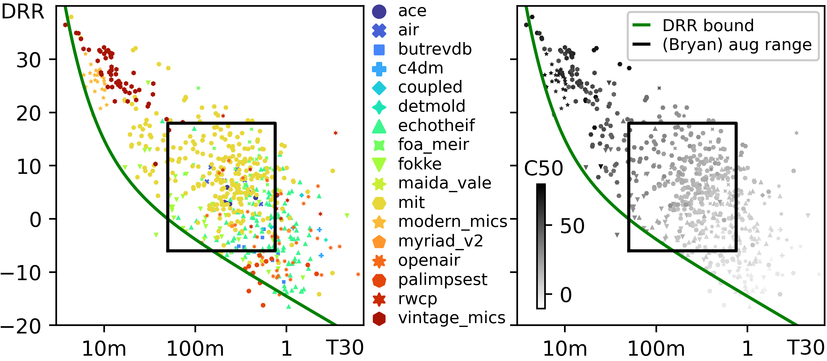
T30 Change. We followed the (Bryan, 2019)'s approach; we multiplied an exponentially decaying window centered to the estimated onset to change T30. The amount of T30 change (in ratio) was sampled from truncated Gaussian, with mean of 0, standard deviation of 0.25, and range of (-0.9, 0.05). We used conservative ratio for the positive ratio since it could amplify the noise floor.
DRR Change. We changed DRR by multiplying the onset-centered 5ms Hann window to estimate the direct arrival, rescaling it, and mixing it with the rest. The DRR change was uniformly sampled from (-12dB, 12dB). However, when the changed DRR is lower than the expected DRR value of exponentially decaying noise with the same T30, we do not reduce the DRR further than that.
Parametric Equalizer. We use 10 second-order sections (biquads), 1 low-shelf filter, 8 peaking filters, and 1 high-shelf filter. Their cutoff frequency is sampled from (60Hz, 20kHz) uniformly under logarithmic scale. The lowest frequency and the highest frequency is assigned to the low-shelf and the high-shelf, respectively. We sample the Q (quality) factor from (0.5, 4) similarly. The gain values are uniformly sampled from (-12dB, 12dB).
Resampling. We sample the sampling rate change from (1/1.5, 1.5), with a truncated Gaussian distribution in a logarithmic scale. That is, we first sample alpha from (-log2(1.5), log2(1.5)), then compute 2^alpha. The mean, standard deviation, and value range of the alpha was 0, log2(1.5)/2, and (-log2(1.5), log2(1.5)). For the IRs with sampling rate lower than 44100 (our main sampling rate), we do not downsampled them.
Channel Mixing. We mix the channel for the multichannel IRs. We uniformly sample the mixing weight from (-1, 1), energy-normalize them, and perform linear combination of the IR signals across the channel.
MicIR. We sometimes convolve MicIRs to change magnitude/phase response and obtain a new IR.